Self Consistency Toy ex

ITSTGCN

Author

SEOYEON CHOI

Published

July 18, 2023

Self Consistency

Tip with Title

Toy example for Self Consistency

Ref: Self Consistency: A General Recipe for Wavelet Estimation With Irregularly-spaced and/or Incomplete Data

Self Consistency : A General Recipe for Wavelet Estimation With Irregularly-spaced and/or Incomplete Data
- 2 Self Consistency: How Does It Work? 2.1 Self-consistency: An Intuitive Principle

\[\mathbb{E}(\hat{f}_{com} | f = \hat{f}_{obs}) = \hat{f}_{obs}\]

Original self-consistency
- \(\hat{f}_{obs} = x_{obs}\) 만 가지고 결측값을 업데이트 한다.
- 이 때, 전제 조건이 필요한데, 결측값을 채우지 않아도 업데이트 가능, 즉 회귀 직선을 구하는 것이 가능해야 했다.
Lee and Meng(위 reference)
- \(\hat{f}_{obs}\)는 missing 값을 가지고 있는 데이터인데, STGCN과 같이 missing 값을 채우지 않으면 모형이 돌아가지 않는 original 의 전제조건을 만족하지 않은 경우가 있다.
- 이 경우에도 임의의 값을 채우고 업데이트함으로써 true regression model에 수렴한다는 것을 밝혔다.

Figure

import numpy as np
import matplotlib.pyplot as plt
import pandas as pd
import copy

T = 10

e = np.random.normal(size=T)*2

x = np.array(range(1,11))

y_true = 2 * x

y = 2 * x + e

y_miss = y.copy()

miss_num = [4,6,7]

y_miss[miss_num] = np.nan

y_miss

array([ 1.27346295,  2.56239243,  8.66405911, 10.22991086,         nan,
       10.79301596,         nan,         nan, 16.94282818, 20.51110477])

with plt.style.context('seaborn-white'):
    plt.figure(figsize=(10,6))
    plt.plot(x,y_miss,'.')
    plt.plot(x,y,'--')
    plt.plot(x,y_true)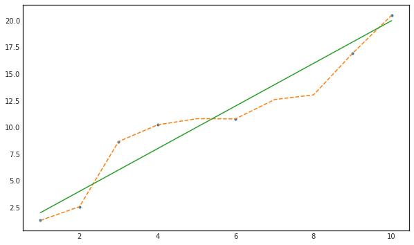

# y_miss_impu = pd.DataFrame(y_miss).interpolate(method='nearest')

y_miss_impu = y_miss.copy()

y_miss_impu[miss_num] = 0

y_miss_impu[miss_num]

array([0., 0., 0.])

y_miss_impu

array([ 1.27346295,  2.56239243,  8.66405911, 10.22991086,  0.        ,
       10.79301596,  0.        ,  0.        , 16.94282818, 20.51110477])

with plt.style.context('seaborn-white'):
    plt.figure(figsize=(10,6))
    plt.plot(x,y_miss_impu,'.')
    plt.plot(x,y,'--')
    plt.plot(x,y_true)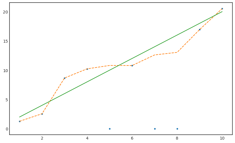

\[\hat{\beta} = \frac{\sum^n_{i=1} y_i x_i}{\sum^n_{i=1} x_i^2}\]

\[\hat{\beta} = \frac{\sum_{i=1}^m y_i x_i + \hat{\beta}_m \sum_{i=m+1}^n x_i^2}{\sum_{i=1}^n x_i^2}\]

y_miss_impu

array([ 1.27346295,  2.56239243,  8.66405911, 10.22991086,  0.        ,
       10.79301596,  0.        ,  0.        , 16.94282818, 20.51110477])

yx_sq = np.sum(y_miss_impu * x);yx_sq

495.6646656336689

x_sq = sum(x**2);x_sq

beta_hat = yx_sq/x_sq

beta_hat

1.2874406899575817

y_iter_zero = beta_hat * x

y_iter_zero

array([ 1.28744069,  2.57488138,  3.86232207,  5.14976276,  6.43720345,
        7.72464414,  9.01208483, 10.29952552, 11.58696621, 12.8744069 ])

y_miss_impu_zero = y_miss_impu.copy()

y_miss_impu_zero[miss_num] = y_iter_zero[miss_num]

y_miss_impu_zero

array([ 1.27346295,  2.56239243,  8.66405911, 10.22991086,  6.43720345,
       10.79301596,  9.01208483, 10.29952552, 16.94282818, 20.51110477])

with plt.style.context('seaborn-white'):
    plt.figure(figsize=(10,6))
    plt.plot(x,y_miss_impu_zero,'.')
    plt.plot(x,y,'--')
    plt.plot(x,y_true)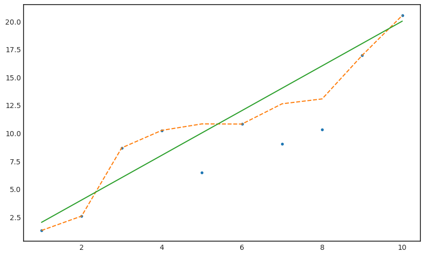

yx_sq_one = sum([y_miss_impu_zero.tolist()] * x);yx_sq_one

array([  1.27346295,   5.12478485,  25.99217733,  40.91964344,
        32.18601725,  64.75809574,  63.08459381,  82.39620416,
       152.48545364, 205.11104769])

beta_hat_iter_one = yx_sq_one/x_sq

beta_hat_iter_one = (beta_hat + beta_hat_iter_one).mean()

y_iter_one = beta_hat_iter_one * x

y_iter_one

array([ 1.46233198,  2.92466397,  4.38699595,  5.84932793,  7.31165992,
        8.7739919 , 10.23632389, 11.69865587, 13.16098785, 14.62331984])

y_iter_one[miss_num]

array([ 7.31165992, 10.23632389, 11.69865587])

y_miss_impu_one = y_miss_impu_zero.copy()

y_miss_impu_one[miss_num] = y_iter_one[miss_num]

with plt.style.context('seaborn-white'):
    plt.figure(figsize=(10,6))
    plt.plot(x,y_miss_impu_one,'.')
    plt.plot(x,y,'--')
    plt.plot(x,y_true)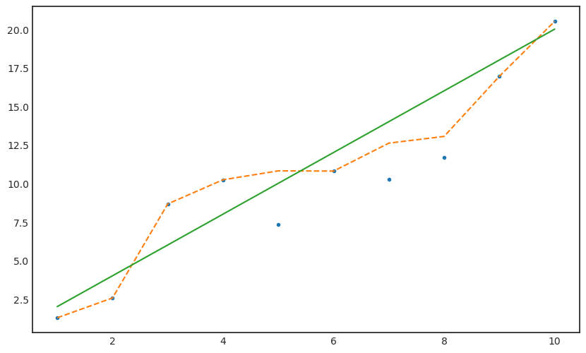

yx_sq_iter_two = sum([y_miss_impu_one.tolist()] * x);yx_sq_iter_two

array([  1.27346295,   5.12478485,  25.99217733,  40.91964344,
        36.55829959,  64.75809574,  71.6542672 ,  93.58924696,
       152.48545364, 205.11104769])

beta_hat_iter_two = yx_sq_iter_two/x_sq

beta_hat_iter_two = (beta_hat_iter_one + beta_hat_iter_two).mean()

y_iter_two = beta_hat_iter_two * x

y_iter_two[miss_num]

array([ 8.21746054, 11.50444476, 13.14793687])

y_miss_impu_two = y_miss_impu_one.copy()

y_miss_impu_two[miss_num,] = y_iter_two[miss_num,]

with plt.style.context('seaborn-white'):
    plt.figure(figsize=(10,6))
    plt.plot(x,y_miss_impu_two,'.')
    plt.plot(x,y,'--')
    plt.plot(x,y_true)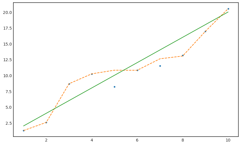

yx_sq_iter_tre = sum([y_iter_two.tolist()] * x);yx_sq_iter_tre

array([  1.64349211,   6.57396843,  14.79142897,  26.29587373,
        41.0873027 ,  59.1657159 ,  80.5311133 , 105.18349492,
       133.12286076, 164.34921082])

beta_hat_iter_tre = yx_sq_iter_tre/x_sq

beta_hat_iter_tre = (beta_hat_iter_two + beta_hat_iter_tre).mean()

y_iter_tre = beta_hat_iter_tre * x

y_iter_tre[miss_num]

array([ 9.0392066 , 12.65488923, 14.46273055])

y_miss_impu_tre = y_miss_impu_two.copy()

y_miss_impu_tre[miss_num] = y_iter_tre[miss_num]

with plt.style.context('seaborn-white'):
    plt.figure(figsize=(10,6))
    plt.plot(x,y_miss_impu_tre,'.')
    plt.plot(x,y,'--')
    plt.plot(x,y_true)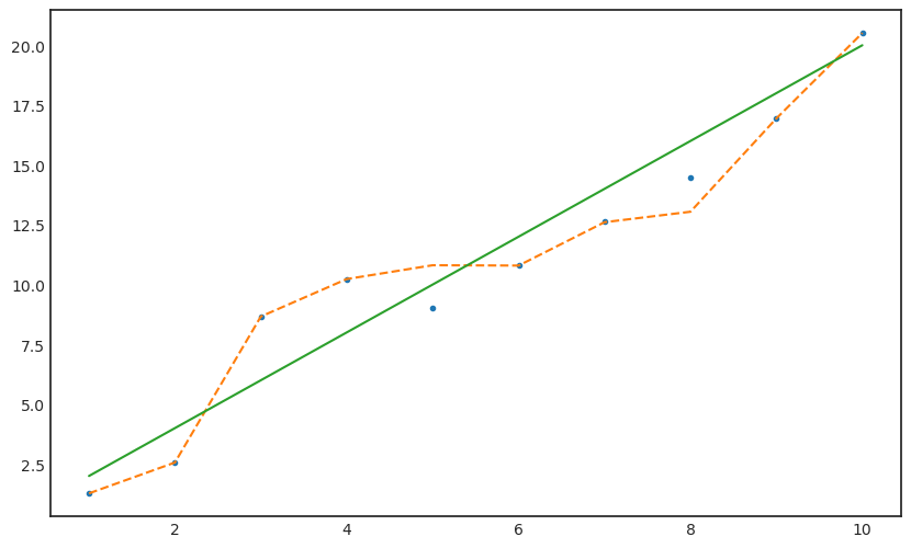

yx_sq_iter_fth = sum([y_iter_tre.tolist()] * x);yx_sq_iter_fth

array([  1.80784132,   7.23136528,  16.27057187,  28.9254611 ,
        45.19603298,  65.08228748,  88.58422463, 115.70184442,
       146.43514684, 180.7841319 ])

beta_hat_iter_fth = yx_sq_iter_fth/x_sq

beta_hat_iter_fth = (beta_hat_iter_tre + beta_hat_iter_fth).mean()

y_iter_fth = beta_hat_iter_fth * x

y_iter_fth[miss_num]

array([ 9.94312725, 13.92037816, 15.90900361])

y_miss_impu_fth = y_miss_impu_tre.copy()

y_miss_impu_fth[miss_num,] = y_iter_fth[miss_num,]

with plt.style.context('seaborn-white'):
    plt.figure(figsize=(10,6))
    plt.plot(x,y_miss_impu_fth,'.')
    plt.plot(x,y,'--')
    plt.plot(x,y_true)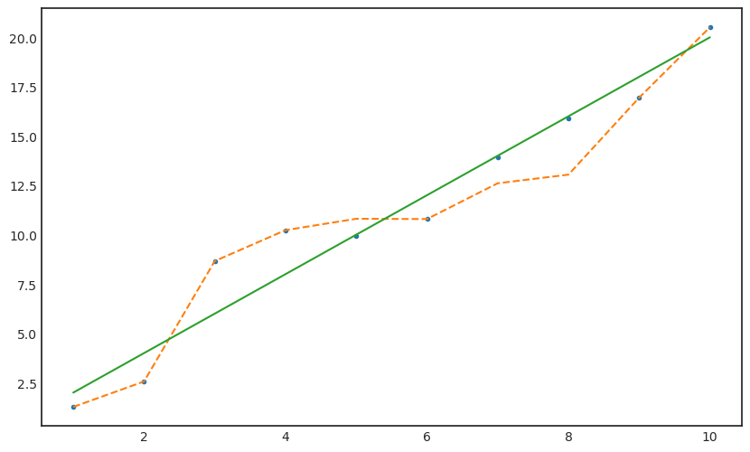

yx_sq_iter_fif = sum([y_iter_fth.tolist()] * x);yx_sq_iter_fif

array([  1.98862545,   7.9545018 ,  17.89762906,  31.81800721,
        49.71563627,  71.59051623,  97.4426471 , 127.27202886,
       161.07866152, 198.86254509])

beta_hat_iter_fif = yx_sq_iter_fif/x_sq

beta_hat_iter_fif = (beta_hat_iter_fth + beta_hat_iter_fif).mean()

y_iter_fif = beta_hat_iter_fif * x

y_iter_fif[miss_num]

array([10.93743998, 15.31241597, 17.49990397])

y_miss_impu_fif = y_miss_impu_fth.copy()

y_miss_impu_fif[miss_num] = y_iter_fif[miss_num]

with plt.style.context('seaborn-white'):
    plt.figure(figsize=(10,6))
    plt.plot(x,y_miss_impu_fif,'.')
    plt.plot(x,y,'--')
    plt.plot(x,y_true)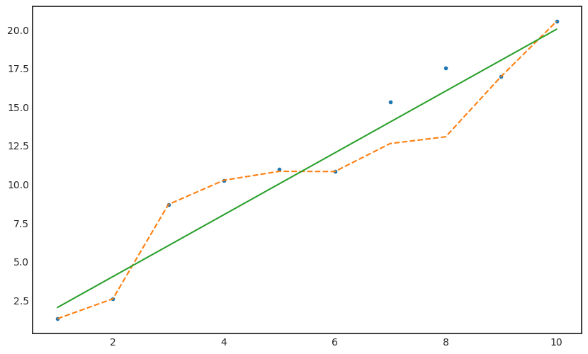

Result

miss_num_1 = [5,7,8]

with plt.style.context('seaborn-white'):
    fig, ax = plt.subplots(figsize=(20,10))
    # fig.suptitle('Figure',fontsize=40)
    plt.tight_layout()
    
    ax.plot(x,y_miss,'o',label='Incomplete Data',markersize=8)
    ax.plot(x,y,'--',color='blue')
    ax.plot(x,y_true,label='True',color='black',alpha=0.5)
    ax.plot(miss_num_1,y_miss_impu[miss_num],'o',color='C3',markersize=8)
    ax.plot(miss_num_1,y_miss_impu_zero[miss_num],'*',color='C3',markersize=8)
    ax.plot(miss_num_1,y_miss_impu_one[miss_num],'*',color='C3',markersize=8)
    ax.plot(miss_num_1,y_miss_impu_two[miss_num],'*',color='C3',markersize=8)
    ax.plot(miss_num_1,y_miss_impu_tre[miss_num],'*',color='C3',markersize=8)
    ax.plot(miss_num_1,y_miss_impu_fth[miss_num],'*',color='C3',markersize=8)
    ax.plot(miss_num_1,y_miss_impu_fif[miss_num],'o',color='C3',markersize=8)
    ax.legend(fontsize=20,loc='upper left',facecolor='white', frameon=True)
    
    # ax.annotate('1st value',xy=(miss_num[0]+0.1,y_miss_impu[miss_num][0]),fontsize=20)
    # ax.annotate('1st value',xy=(miss_num[1]+0.1,y_miss_impu[miss_num][1]),fontsize=20)
    # ax.annotate('1st value',xy=(miss_num[2]+0.1,y_miss_impu[miss_num][2]),fontsize=20)
    # ax.annotate('5th iteration',xy=(miss_num[0]+0.1,y_miss_impu_fif[miss_num][0]),fontsize=20)
    # ax.annotate('5th iteration',xy=(miss_num[1]+0.1,y_miss_impu_fif[miss_num][1]),fontsize=20)
    # ax.annotate('5th iteration',xy=(miss_num[2]+0.1,y_miss_impu_fif[miss_num][2]),fontsize=20)
    
    # ax.arrow(miss_num[0]+0.4, y_miss_impu[miss_num][0]+0.6, 0, y_miss_impu_fif[miss_num][0]-1.5,linestyle= 'dashed', head_width=0.1, head_length=0.3, fc='black',ec='black',alpha=0.5)
    # ax.arrow(miss_num[1]+0.4, y_miss_impu[miss_num][1]+0.6, 0, y_miss_impu_fif[miss_num][1]-1.5,linestyle= 'dashed', head_width=0.1, head_length=0.3, fc='black',ec='black',alpha=0.5)
    # ax.arrow(miss_num[2]+0.4, y_miss_impu[miss_num][2]+0.6, 0, y_miss_impu_fif[miss_num][2]-1.5,linestyle= 'dashed', head_width=0.1, head_length=0.3, fc='black',ec='black',alpha=0.5)

    # ax.plot(miss_num, y_miss_impu[miss_num], 'o', markersize=30, markerfacecolor='none', markeredgecolor='red',markeredgewidth=1,color='C4')
    
    ax.tick_params(axis='y', labelsize=20)
    ax.tick_params(axis='x', labelsize=20)
# plt.savefig('Self_consistency_Toy.png')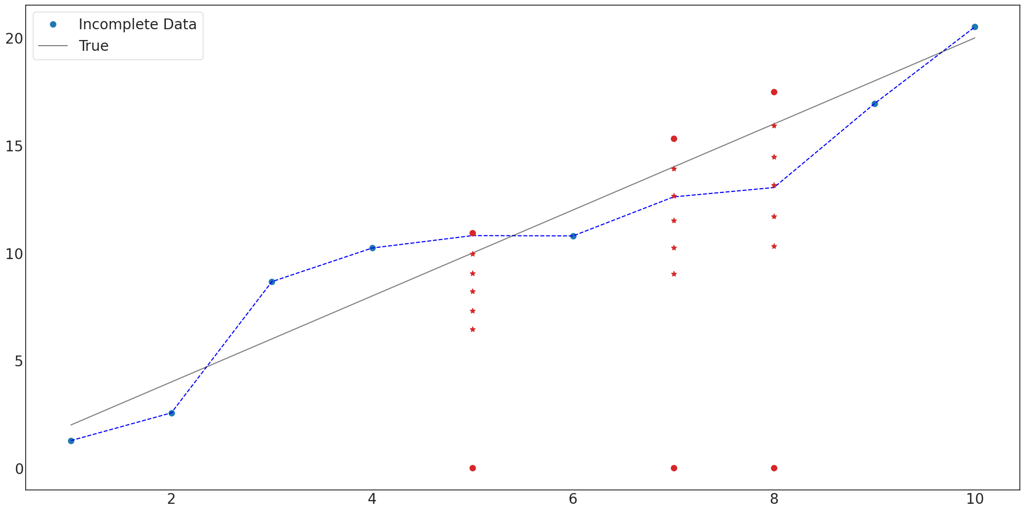

with plt.style.context('seaborn-white'):
    fig, ax = plt.subplots(figsize=(20,10))
    # fig.suptitle('Figure',fontsize=40)
    plt.tight_layout()
    
    ax.plot(x,y_true,label='True',color='black',alpha=0.5)
    ax.plot(x,y_miss,'o',label='$x_{obs}$',markersize=8)
    # ax.plot(x,y,'--',color='blue')
    
    # ax.plot(x,y_iter_zero)
    # ax.plot(x,y_iter_one)
    # ax.plot(x,y_iter_two)
    # ax.plot(x,y_iter_tre)
    ax.plot(x,y_iter_fth,color='blue',alpha=0.5,label='$\hat{f}_{obs}$')
    # ax.plot(x,y_iter_fif)
    ax.plot(miss_num_1,y_miss_impu[miss_num],'o',color='C3',markersize=8)
    ax.plot(miss_num_1,y_miss_impu_zero[miss_num],'*',color='C3',markersize=8)
    ax.plot(miss_num_1,y_miss_impu_one[miss_num],'*',color='C3',markersize=8)
    ax.plot(miss_num_1,y_miss_impu_two[miss_num],'*',color='C3',markersize=8)
    ax.plot(miss_num_1,y_miss_impu_tre[miss_num],'*',color='C3',markersize=8)
    ax.plot(miss_num_1,y_miss_impu_fth[miss_num],'o',color='C3',markersize=8)
    # ax.plot(miss_num,y_miss_impu_fif[miss_num],'o',color='C3',markersize=8)
    
    ax.legend(fontsize=20,loc='upper left',facecolor='white', frameon=True)
    
    ax.annotate('1st value',xy=(miss_num_1[0]+0.1,y_miss_impu[miss_num][0]),fontsize=20)
    ax.annotate('1st value',xy=(miss_num_1[1]+0.1,y_miss_impu[miss_num][1]),fontsize=20)
    ax.annotate('1st value',xy=(miss_num_1[2]+0.1,y_miss_impu[miss_num][2]),fontsize=20)
    ax.annotate('5th iteration',xy=(miss_num_1[0]+0.1,y_miss_impu_fth[miss_num][0]-0.3),fontsize=20)
    ax.annotate('5th iteration',xy=(miss_num_1[1]+0.1,y_miss_impu_fth[miss_num][1]-0.3),fontsize=20)
    ax.annotate('5th iteration',xy=(miss_num_1[2]+0.1,y_miss_impu_fth[miss_num][2]-0.3),fontsize=20)
    
    ax.arrow(miss_num_1[0]+0.4, y_miss_impu[miss_num][0]+0.6, 0, y_miss_impu_fth[miss_num][0]-1.5,linestyle= 'dashed', head_width=0.1, head_length=0.3, fc='black',ec='black',alpha=0.5)
    ax.arrow(miss_num_1[1]+0.4, y_miss_impu[miss_num][1]+0.6, 0, y_miss_impu_fth[miss_num][1]-1.5,linestyle= 'dashed', head_width=0.1, head_length=0.3, fc='black',ec='black',alpha=0.5)
    ax.arrow(miss_num_1[2]+0.4, y_miss_impu[miss_num][2]+0.6, 0, y_miss_impu_fth[miss_num][2]-1.5,linestyle= 'dashed', head_width=0.1, head_length=0.3, fc='black',ec='black',alpha=0.5)

    # ax.plot(miss_num_1, y_miss_impu[miss_num], 'o', markersize=30, markerfacecolor='none', markeredgecolor='red',markeredgewidth=1,color='C4')
    
    ax.tick_params(axis='y', labelsize=20)
    ax.tick_params(axis='x', labelsize=20)
plt.savefig('Self_consistency_Toy_0617.png')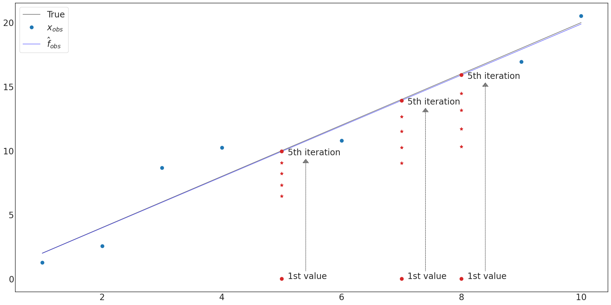

Theory

2 Self Consistency: How Does It Work?

2.1 Self-consistency: An Intuitive Principle

책에서의 가정

\(x = 0,1,2,3,\dots,16\)으로 fixed 되어 있음.
\(y_0,\dots, y_{13}\)까지의 값을 알고 있는데 \(y_{14},y_{15},y_{16}\)의 값은 모른다.

\(y_i=\beta x_i + \epsilon_i, i=1,\dots,n, \epsilon_i \sim \text{i.i.d.}F(0,\sigma^2)\)

\(\beta\)의 최소제곱추정치

\(\hat{\beta}_n = \hat{\beta}_n(y_1 ,\dots,y_n) = \frac{\sum^n_{i=1} y_i x_i}{\sum^n_{i=1} x_i^2}\)

단, \(m<n\) 이고, \(\sum ^n_{m+1} x_i^2 > 0\) 일 때,

\(E(\hat{\beta}_n|y_a, \dots,y_m,;\beta = \hat{\beta}_m) = \hat{\beta}_m\)

the least-squares estimator has a (Martingale-like property)¹, and reaches a perfect equilibrium in its projective properties

¹ 확률 과정 중 과거의 정보를 알고 있다면 미래의 기댓값이 현재값과 동일한 과정

참고;(위키백과)[https://ko.wikipedia.org/wiki/%EB%A7%88%ED%8C%85%EA%B2%8C%EC%9D%BC]

\(\beta_n\)을 구한다.
\(\beta_n \times x\) 를 구한다.
missing 값이 있는 index만 대체한다.
다시 \(\beta_n\)을 구한다.
.. 반복

\(\beta\)의 선형성 때문에 가능한 이론

아래 계산하면 맞아야 함

\(\hat{\beta}_n = \frac{\sum_{i=1}^m y_i x_i + \hat{\beta}_m \sum_{i=m+1}^n x_i^2}{\sum_{i=1}^n x_i^2}\)

2.2 A Self–consistent Regression Estimator

목적은 최적의 \(\hat{f}_{com}\) 찾는 것, 일단 이 paper는 웨이블릿에 중점을 두고 비모수, 준모수 회귀로 확장 가능 누적 분포 함수 CDF 찾는 것이 목적

Fig for Paper

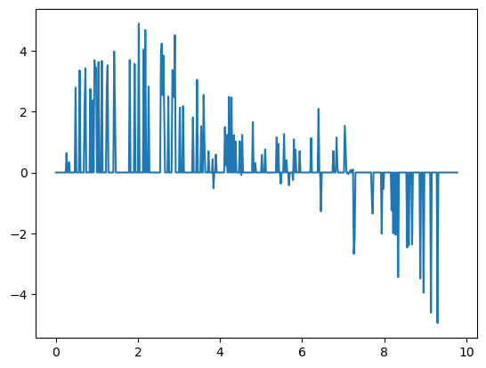
T = 500

t = np.arange(T)/T * 10

y_true = 3*np.sin(0.5*t) + 1.2*np.sin(1.0*t) + 0.5*np.sin(1.2*t) 

y = y_true + np.random.normal(size=T)

plt.figure(figsize=(20,10))
plt.plot(t,y_true,color='red',label = 'true')
plt.plot(t,y,'',color='black',label = 'f')
plt.legend(fontsize=15,loc='lower left',facecolor='white', frameon=True)
# plt.savefig('1.png')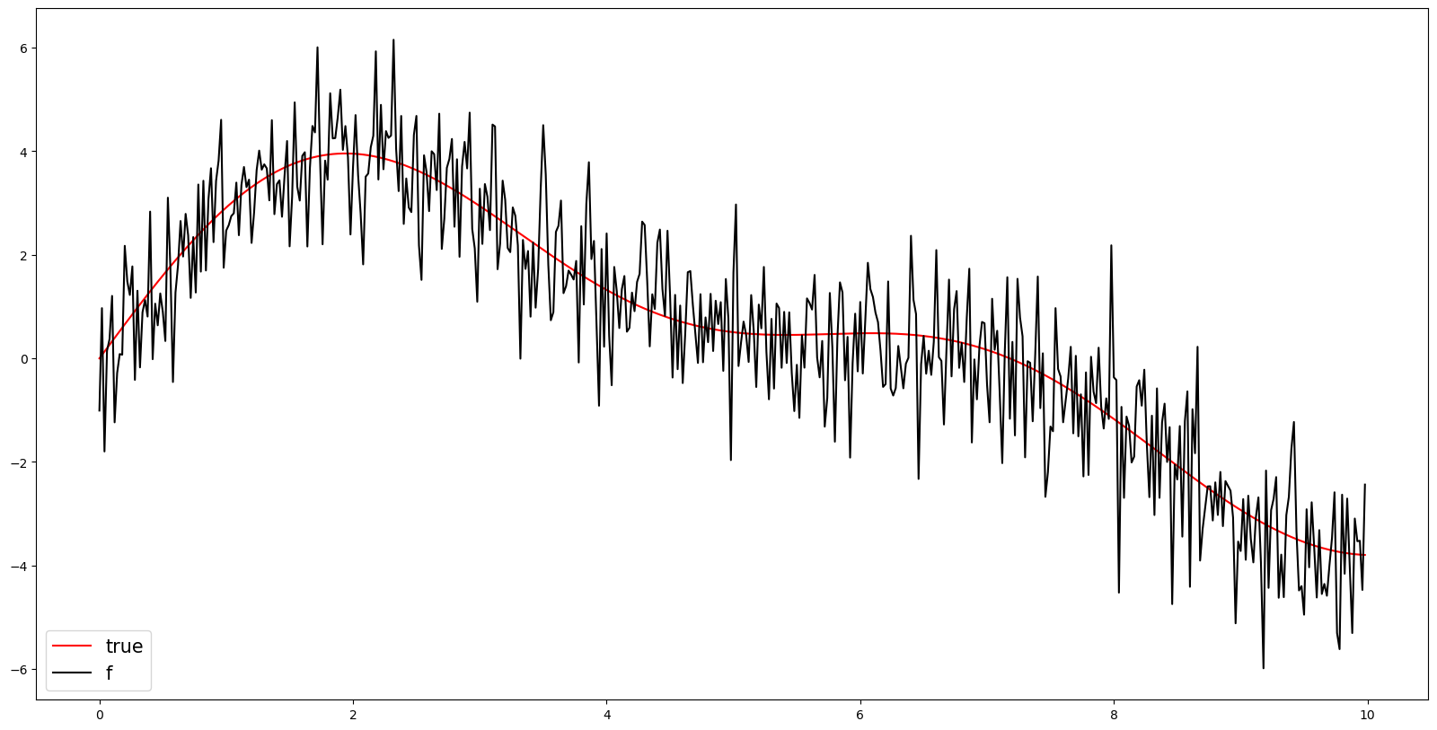

random_num = np.random.choice(range(500), size=400, replace=False)

y[random_num] = np.nan

plt.figure(figsize=(20,10))
plt.plot(t,y_true,color='red',label = 'true')
plt.plot(t,y,'.',color='black',label = 'f')
plt.legend(fontsize=15,loc='lower left',facecolor='white', frameon=True)
# plt.savefig('1.png')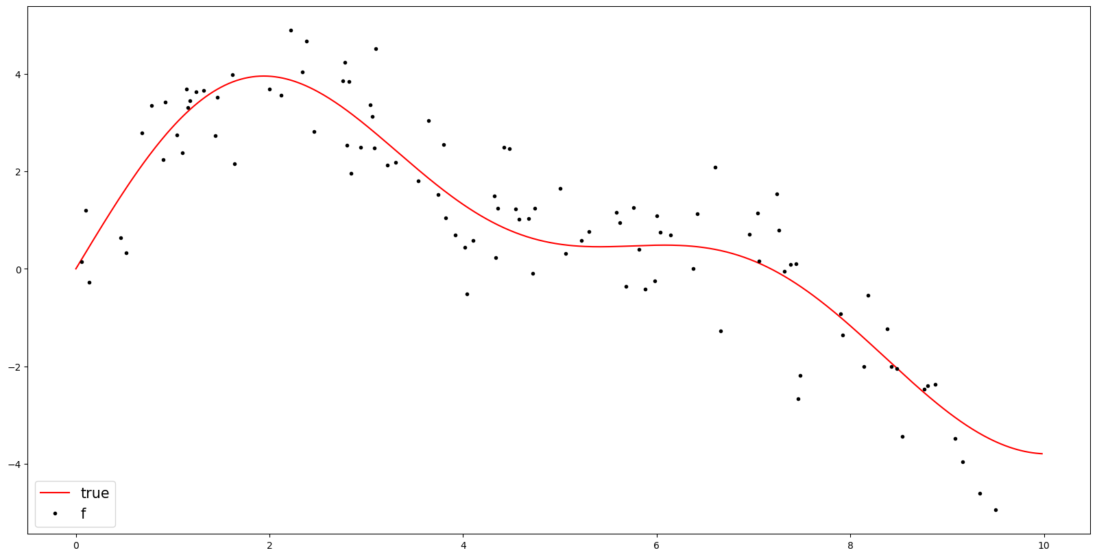

y[random_num] = 0

plt.figure(figsize=(20,10))
plt.plot(t,y_true,color='red',label = 'true')
plt.plot(t,y,'.',color='black',label = 'f')
plt.legend(fontsize=15,loc='lower left',facecolor='white', frameon=True)
# plt.savefig('1.png')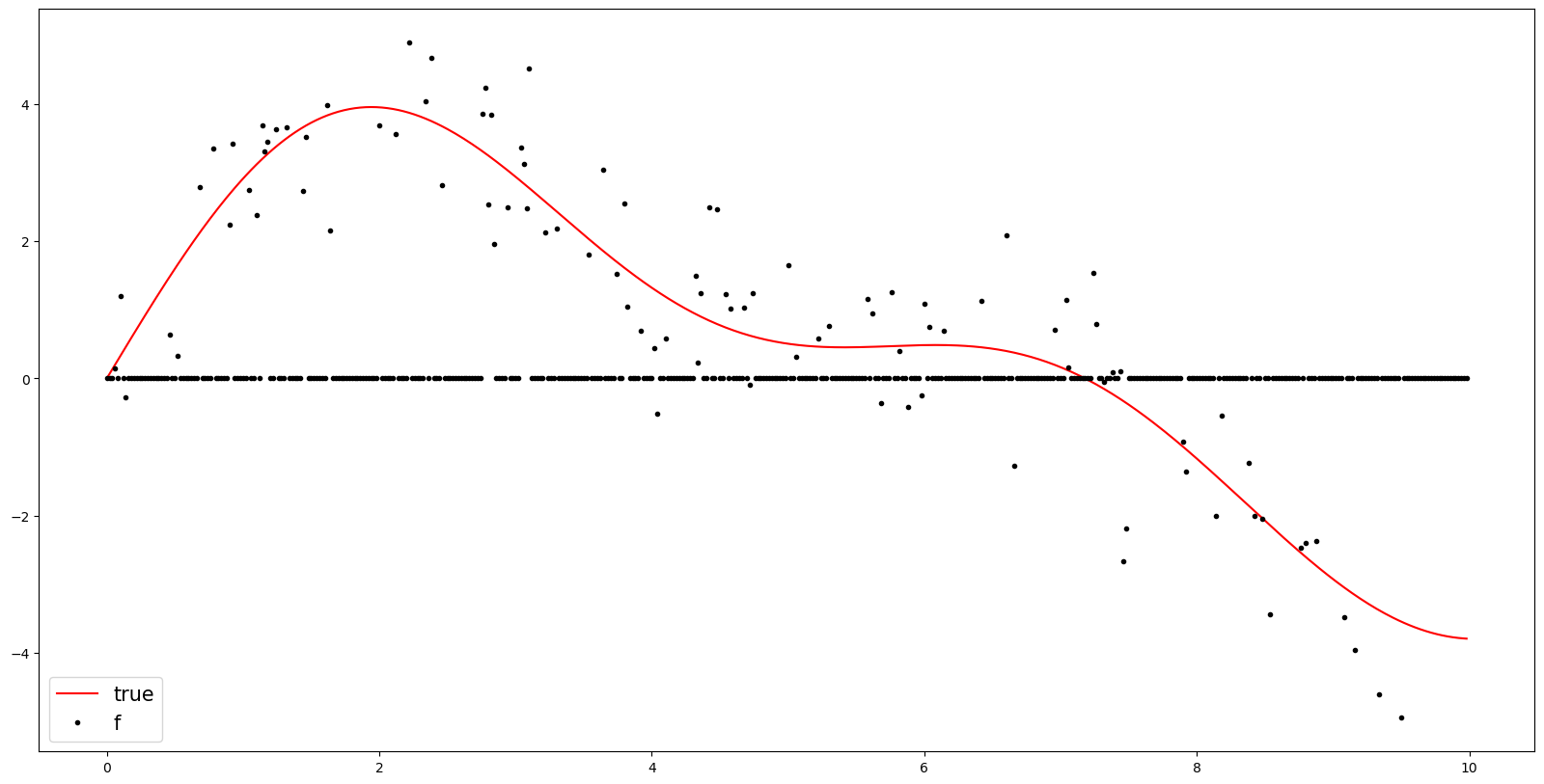

y_inter = pd.DataFrame(y).interpolate(method='linear').fillna(method='bfill').fillna(method='ffill').to_numpy().tolist()

plt.figure(figsize=(20,10))
plt.plot(t,y_true,color='red',label = 'true')
plt.plot(t,y,'.',color='black',label = 'f')
plt.plot(t,y_inter,color = 'blue')
plt.legend(fontsize=15,loc='lower left',facecolor='white', frameon=True)
# plt.savefig('1.png')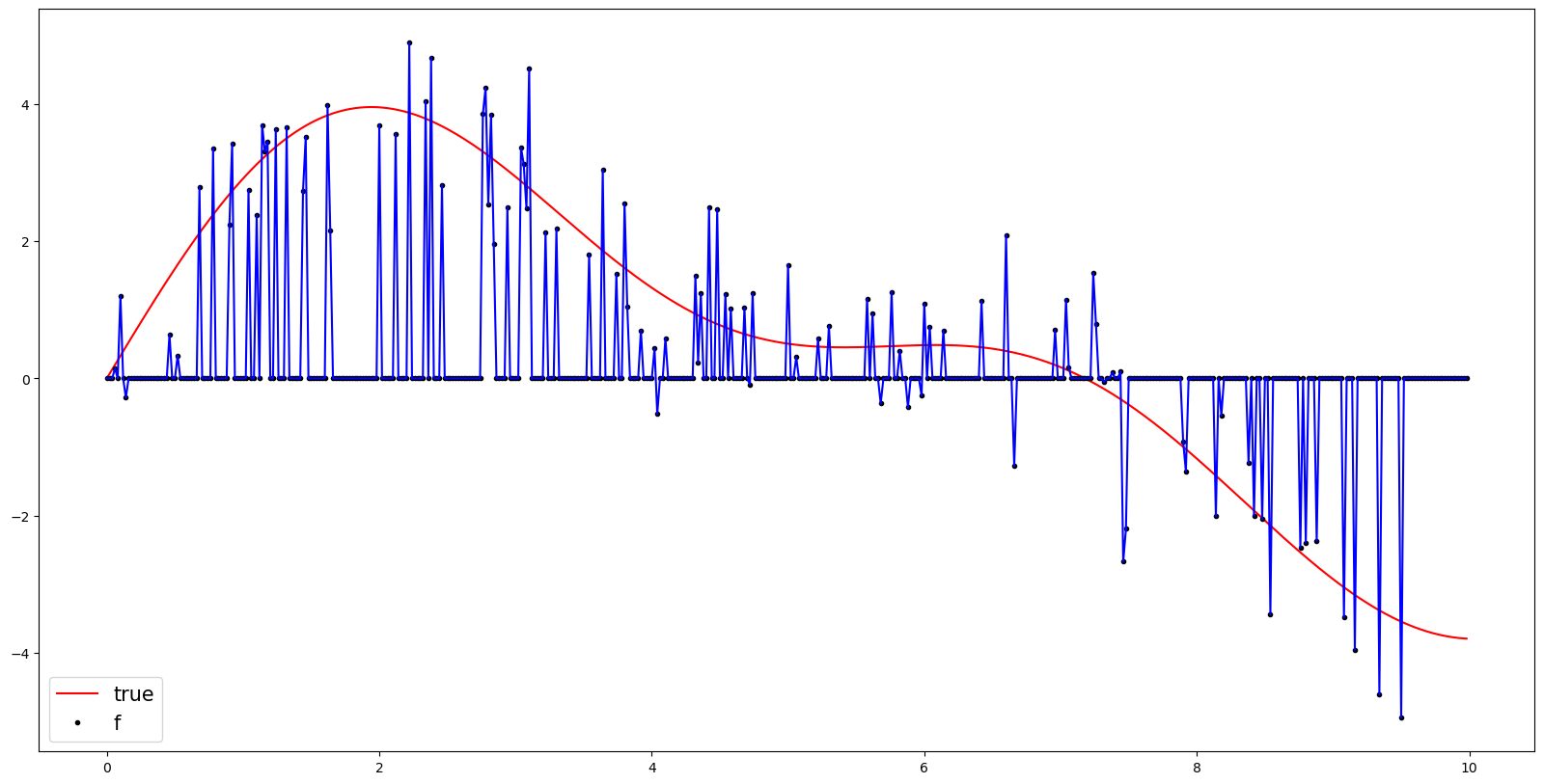

np.array(y_inter).reshape(-1)[random_num]

array([0., 0., 0., 0., 0., 0., 0., 0., 0., 0., 0., 0., 0., 0., 0., 0., 0.,
       0., 0., 0., 0., 0., 0., 0., 0., 0., 0., 0., 0., 0., 0., 0., 0., 0.,
       0., 0., 0., 0., 0., 0., 0., 0., 0., 0., 0., 0., 0., 0., 0., 0., 0.,
       0., 0., 0., 0., 0., 0., 0., 0., 0., 0., 0., 0., 0., 0., 0., 0., 0.,
       0., 0., 0., 0., 0., 0., 0., 0., 0., 0., 0., 0., 0., 0., 0., 0., 0.,
       0., 0., 0., 0., 0., 0., 0., 0., 0., 0., 0., 0., 0., 0., 0., 0., 0.,
       0., 0., 0., 0., 0., 0., 0., 0., 0., 0., 0., 0., 0., 0., 0., 0., 0.,
       0., 0., 0., 0., 0., 0., 0., 0., 0., 0., 0., 0., 0., 0., 0., 0., 0.,
       0., 0., 0., 0., 0., 0., 0., 0., 0., 0., 0., 0., 0., 0., 0., 0., 0.,
       0., 0., 0., 0., 0., 0., 0., 0., 0., 0., 0., 0., 0., 0., 0., 0., 0.,
       0., 0., 0., 0., 0., 0., 0., 0., 0., 0., 0., 0., 0., 0., 0., 0., 0.,
       0., 0., 0., 0., 0., 0., 0., 0., 0., 0., 0., 0., 0., 0., 0., 0., 0.,
       0., 0., 0., 0., 0., 0., 0., 0., 0., 0., 0., 0., 0., 0., 0., 0., 0.,
       0., 0., 0., 0., 0., 0., 0., 0., 0., 0., 0., 0., 0., 0., 0., 0., 0.,
       0., 0., 0., 0., 0., 0., 0., 0., 0., 0., 0., 0., 0., 0., 0., 0., 0.,
       0., 0., 0., 0., 0., 0., 0., 0., 0., 0., 0., 0., 0., 0., 0., 0., 0.,
       0., 0., 0., 0., 0., 0., 0., 0., 0., 0., 0., 0., 0., 0., 0., 0., 0.,
       0., 0., 0., 0., 0., 0., 0., 0., 0., 0., 0., 0., 0., 0., 0., 0., 0.,
       0., 0., 0., 0., 0., 0., 0., 0., 0., 0., 0., 0., 0., 0., 0., 0., 0.,
       0., 0., 0., 0., 0., 0., 0., 0., 0., 0., 0., 0., 0., 0., 0., 0., 0.,
       0., 0., 0., 0., 0., 0., 0., 0., 0., 0., 0., 0., 0., 0., 0., 0., 0.,
       0., 0., 0., 0., 0., 0., 0., 0., 0., 0., 0., 0., 0., 0., 0., 0., 0.,
       0., 0., 0., 0., 0., 0., 0., 0., 0., 0., 0., 0., 0., 0., 0., 0., 0.,
       0., 0., 0., 0., 0., 0., 0., 0., 0.])

import tensorflow as tf
from tensorflow.keras.models import Sequential
from tensorflow.keras.layers import LSTM, Dense

# Define the number of time steps for the LSTM model
time_steps = 10

# Create input and output sequences by shifting the data
X = []
Y = []
for i in range(len(y) - time_steps):
    X.append(y[i:i+time_steps])
    Y.append(y[i+time_steps])

# Convert the sequences to numpy arrays
X = np.array(X)
Y = np.array(Y)

# Reshape the input data to match the LSTM input shape
X = np.reshape(X, (X.shape[0], X.shape[1], 1))

# Define the LSTM model
model = Sequential()
model.add(LSTM(32, input_shape=(time_steps, 1)))
model.add(Dense(1))

# Compile the model
model.compile(loss='mean_squared_error', optimizer='adam')

# Train the model
model.fit(X, Y, epochs=1, batch_size=32)

16/16 [==============================] - 2s 5ms/step - loss: 1.0766

<keras.callbacks.History at 0x7fa83818bdf0>

np.array(Y).reshape(-1)[random_num]

IndexError: index 492 is out of bounds for axis 0 with size 490

plt.plot(t[:490],Y)